00.Networks

Networks

A network is represented by a graph with $N$ nodes (or vertices) and $L$ links (or edges).

• Undirected Networks: No direction associated with links.
• Directed Networks: Links have a specified direction.
• Weighted Networks: Links have weights representing the strength or capacity of the connection.

Adjacency and Laplacian matrices

Representation of networks using the adjacency matrix $A$ is popular. We simply put a $1$ in position $ij$ if exists a link between node $i$ and node $j$, $0$ otherwise. Typically $A$ is a sparse matrix (small density).

A weighted network is described by the $N\times N$ weight matrix $W=w_{ij}$ where $w_{ij}>0$ if the link $i\to j$ exists, $w_{ij}=0$ otherwise.

The $N\times N$ Laplacian matrix is an alternative representation of the network, given by: $L=\text{diag}\left(k_1,k_2,\dots ,k_N\right)-A$

It’s symmetric and zero-row-sum.

Bipartite network

Bipartite networks are made up of two different classes of nodes. Each class has a certain number of nodes. Only nodes from different classes can be connected to each other.

For example, in a network of papers and authors, a paper node can only be connected to an author node, and vice versa.

To represent a bipartite network, we can use a rectangular incidence matrix called $B$.

We can also create a projected network by projecting the bipartite network onto one of the classes of nodes, denoted as $S$. In this projected network, the weight of a link between two nodes is determined by the number of common neighbours they have in the original network.

To obtain the weight matrix $W$ of the projected network, follow these steps:

1. Compute $M=B^{T}B$, where $B^T$ is the transpose of matrix $B$. This multiplication will give an intermediate matrix $M$.
2. Set the diagonal entries of $M$ to zero.

This resulting matrix $M$ will correspond to the weight matrix $W$ of the projected network.

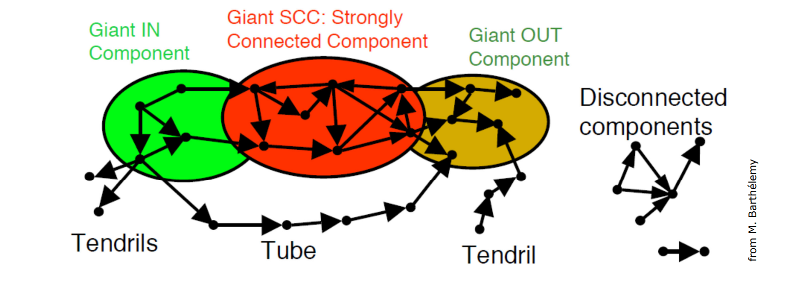
Strongly connected component

It is common to classify components based on their specific properties or the extent of their connectivity. We often refer to highly interconnected sub-sections of a graph as “Strongly Connected Components” or “Giant Out Components” indicating intensive links and relations among its nodes. At the same time, certain components might demonstrate no connectivity or weak connections, forming what we describe as “Disconnected Components”.

Algorithm:

1. For each node of the directed graph check if it’s in “communication” with each other node. Where communication means that $x$ must have a path to $y$ but also $y$ must have one to $x$ (the graph is directed)

After finding the SCC we can also identify:

• in: set of nodes with links that are pointing to the SCC
• out: set of nodes with links that are reachable from the SCC
• tubes: links that are connecting nodes in the in set with nodes of out set

Basic properties

1. For each node of the directed graph check if it’s in “communication” with each other node. Where communication means that $x$ must have a path to $y$ but also $y$ must have one to $x$ (the graph is directed)

The Distance is the length (in number of links) of the shortest path connecting two nodes $i$ and $j$, denoted as $d_{ij}$. We can define:

Diameter (D):

$D=\max (d_{ij})$

The Average Distance (d) $d=\frac{1}{N(N-1)}{\sum }_{i\ne j}{d}_{ij}$

And the Efficiency : $E=⟨\frac{1}{d_{ij}}⟩=\frac{1}{N(N-1)}{\sum }_{i\ne j\in V}\frac{1}{d_{ij}}$ with $\frac{1}{d_{ij}}=0$ if path $i\to j$ does not exist:

“An unconnected pair contributes $0$ to the efficiency of the network”

Density

The density of a network:

$\rho =\frac{L}{N(N-1)}\text{ (dir.) or }\rho =\frac{L}{N(N-1)/2}\text{ (undir.). }$

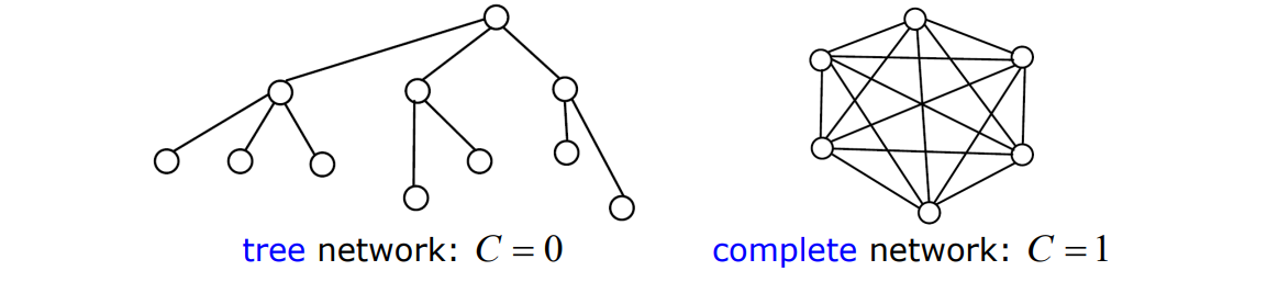
Clustering

Clustering (or Transitivity) Coefficient quantifies “local link density” by counting the triangles in the network. Local Clustering Coefficient $c_i$ of node $i$: $c_i=\frac{e_i}{\frac{k_i(k_i-1)}{2}}$

Where $k_i$ is the degree of $i$ and $e_i$ the number of links directly connecting neighbors of $i$.

The global clustering coefficient is calculated by averaging individual node coefficients $C=⟨c_i⟩$. Global clustering coefficient of a tree is zero (think of the triangles):

Examples:

Network	Size	Clustering coefficient	Average path length
Internet, domain level [13]	32711	0.24	3.56
Internet, router level [13]	228298	0.03	9.51
WwW [14]	153127	0.11	3.1
E-mail [15]	56969	0.03	4.95
Software [16]	1376	0.06	6.39
Electronic circuits [17]	329	0.34	3.17
Language [18]	460902	0.437	2.67
Movie actors [5, 7]	225226	0.79	3.65
Math. co-authorship [19]	70975	0.59	9.50
Food web [20, 21]	154	0.15	3.40
Metabolic system [22]	778	-	3.2

Degree Distribution in Networks

Let’s start with the Degree and Strength of a Node:

• Degree $k_i$ in undirected network is the number of links connected to node $i$.
• Strength $s_i$ in a weighted network is the total weight of the links connected to node $i$.

In a directed network we can distinct in,out and total degree/strength.

The **Degree Distribution $P(k)$ of a network is the fraction of nodes having exactly degree $k$.

$P(k)=\frac{\text{ Number of nodes with degree }k}{N},{\sum }_{k}P(k)=1$

It is often more practical to consider the Cumulative Degree Distribution which is the fraction of nodes with degree $\ge k$:

$\bar{P}(k)=\frac{\text{ Number of nodes with degree }\ge k}{N}={\sum }_{h=k}^{k_{\max }}P(h),\bar{P}\left(k_{\min }\right)=1$

And the moments of Degree Distribution: $⟨k^r⟩$ are:

$<k^r>={\sum }_k{k}^{r}P(k),r=1,2,\dots$

The first moment $(r=1)$ is the average degree $<k>={\sum }_{k}kP(k)=\frac{1}{N}$which interestingly can be also computed as

$<k>={\sum }_i{k}_i=\frac{2L}{N}$

Authorities and hubs

Homogeneous Network: All nodes have the same degree. Heterogeneous Network (Real-World): Broad degree distribution, some nodes are highly connected (hubs), while most have few connections.

Said this we can talk about authorities and hubs scores which are based taking into account the different role of in-out links. The formulas of authorities and hubs score are part of a recursive process: the authority score of a node depends on the hub scores of nodes pointing to it, and the hub score of a node depends on the authority scores of the nodes it points to. This interdependency is key in networks where the importance of a node is not just a function of how many connections it has, but also how important those connections are.

Authority Score $x_i$ :

$x_i=\alpha {\sum }_j{a}_{ji}{y}_j$

The authority score is calculated by summing the hub scores $y_j$ of all nodes $j$ that point to $i$. The adjacency matrix $a_{ji}$ is used to know if there’s a link from node $j\to i$ . The factor $\alpha$ is a normalization constant to keep the scores from escalating too high.

Hub Score $y_i$:

$y_i=\beta {\sum }_j{a}_{ij}{x}_j$

The hub score $y_i$ of a node $i$ is computed by summing the authority scores $x_j$ of all nodes $j$ that node $i$ points to. The adjacency matrix $a_{ij}$ indicates whether there is a link from node $i\to j$. The factor $\beta$ serves as a normalization constant to prevent the scores from becoming excessively large.

Nearest neighbors

The degree distribution of nearest neighbours $Q(h)$ specifies the fraction of nodes’ neighbours having exactly degree $h$ (=the probability that a randomly selected neighbour of a randomly selected node has degree $h$ ):

It is not $P(k)$ but it is biased towards highest degrees:

$Q(h)=\frac{\text{ n. of links from nodes of degree }h}{\text{ n. of links from nodes of any degree }}=\frac{h(P(h)N)}{{\sum }_{k}k(P(k)N)}=\frac{hP(h)}{<k>}$

Thus the average degree of nearest neighbours $k_{nn}$ is:

$k_{nn}={\sum }_{h}hQ(h)={\sum }_h\frac{h^{2}P(h)}{<k>}=\frac{<k^2>}{<k>}=\frac{<k{>}^2+{\sigma }^2}{<k>}=<k>+\frac{{\sigma }^2}{<k>}$

which is larger than $<k>$ provided ${\sigma }^2\ne 0$ (non strictly homogeneous network).

If variance is not equal to zero, $Q(h)$ is always higher than $P(k)$ .

This is the mathematical foundation of the friendship paradox which states that on average, your friends will have more friends than you do. As navigating randomly through a network is more likely to encounter nodes with many connections. This idea has applications for finding hub nodes within a network.

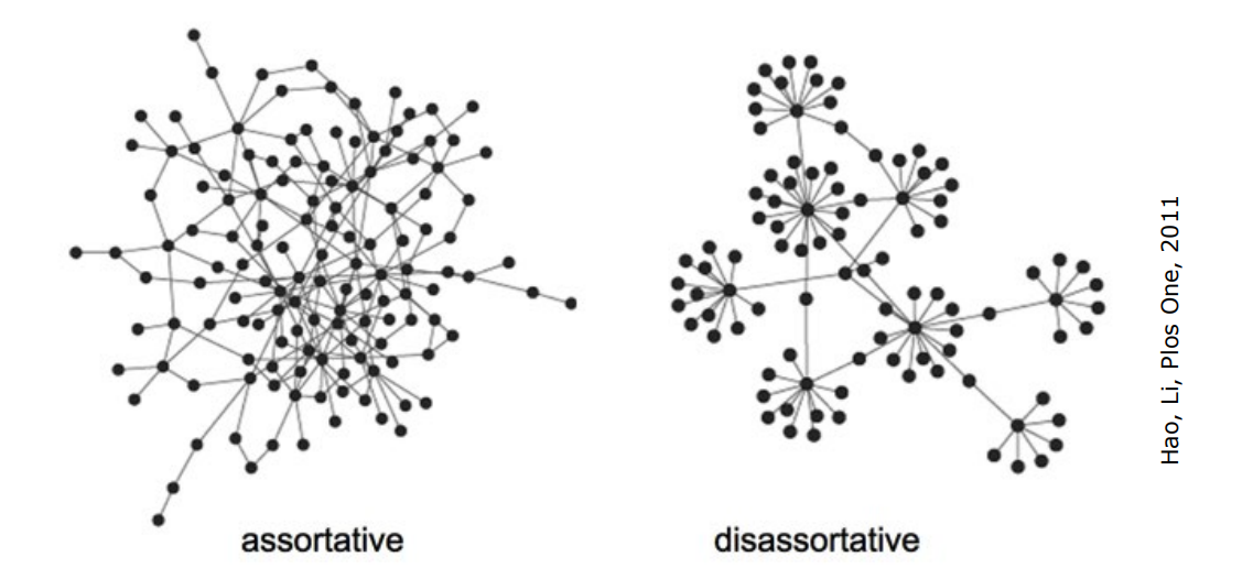
Correlated Networks

There is a correlation between $P(k)$ with $Q(k)$? In a degree-correlated network, the probability $P(h|k)$ that the neighbour of a node with degree $k$ has degree $h$ depends on $k$. Correlations in such a network can be captured by the average nearest neighbour degree function: $k_{nn}(k)={\sum }_{h}hP(h|k)$ Practically, this function is computed as: $k_{nn}(k)=\frac{1}{N(k)}{\sum }_{i|k_i=k}\frac{1}{k}{\sum }_j{a}_{ij}{k}_j$ where $N(k)$ is the number of nodes with degree $k$. In an assortative network, high-degree nodes tend to connect to other high-degree nodes. Conversely, in a disassortative network, high-degree nodes tend to connect to low-degree nodes.

In an assortative network, high-degree nodes tend to connect to other high-degree nodes. Conversely, in a disassortative network, high-degree nodes tend to connect to low-degree nodes.

In summary, $k_{nn}(k)$ provides insight into the degree correlation patterns within a network, revealing how nodes of a certain degree tend to connect with other nodes of specific degrees.

Random walks on networks

A random walk is a path formed by a sequence of random steps. Random walks have many variants:

• Discrete vs continuous time
• Uniform vs non-uniform steps
• Markovian vs non-Markovian processes
• etc.

Random walks have practically unlimited applications across all scientific fields: ecology, economics, psychology, computer science, physics, chemistry, and biology.

In a unweighted network, the random walker at node $i$ chooses an out-link $i\to j$ with uniform probability:

$p_{ij}=\frac{a_{ij}}{k_i^{\text{out}}}$

In a weighted network, the out-link is chosen with probability proportional to its weight:

$p_{ij}=\frac{w_{ij}}{{\sum }_j{w}_{ij}}=\frac{w_{ij}}{s_i^{\text{out}}}$

The transition matrix $P=\left[p_{ij}\right]$ is the $N\times N$ matrix which represents the probabilities of a random walker moving from node $i$ to any node $j$. The probabilities are not symmetric because each row is normalized with $k_i^{\text{at}}$.

${\pi }_{i,t}=$ state probability $=$ probability of being in node $i$ at time $t$ $({\sum }_i{\pi }_{i,t}=1\forall t)$. ${\pi }_t=\left(\begin{array}{llll}{\pi }_{1,t}& {\pi }_{2,t}& \cdots & {\pi }_{N,t}\end{array}\right)$ evolves according to the Markov chain equation:

${\pi }_{t+1}={\pi }_{t}P,{\pi }_{i,t+1}={\sum }_{n=1}^N{\pi }_{n,t}{p}_{ni}$

If the network is strongly connected, then:

• The transition matrix $P=\left[p_{ij}\right]$ is irreducible.
• There exists a unique stationary state probability distribution $\pi =\pi P$, which is strictly positive $({\pi }_i>0$ for all $i)$.

${\pi }_i=\text{fraction of time spent on node }i=\text{centrality of node }i$

Observations:

• In undirected networks, ${\pi }_i$ is the (rescaled) node strength: ${\pi }_i=s_i/{\sum }_j{s}_j$.
• In directed networks, ${\pi }_i$ is mostly correlated to the in-strength $s_i^{\text{in}}$ (e.g., WWW).

Google PageRank

The solution to $\pi =\pi P$ might not be unique, positive, or the Markov chain might not even be well-defined. PageRank uses teleportation: at each time step, the random walker has a probability $\gamma >0$ to jump to a randomly selected node.

$p_{ij}\to p_{ij}^{\prime }=(1-\gamma )\frac{w_{ij}}{s_i^{\text{out}}}+\gamma \frac{1}{N}$

A suitable value for $\gamma$ is not too large (to avoid heavily modifying the network) nor too small (to prevent ${\pi }_i$ from being too sensitive to $\gamma$). The standard (Google) value is $\gamma =0.15$.

PageRank’s revolution is that the rank emerges naturally from the self-organized internet structure. A high rank is achieved only if many other nodes point to it, creating a naturally emerged rank.

Node centrality

The centrality of a node is a measure of its importance in the network. The importance of a node can trivially be captured by the number $k_i$ of its neighbours (or in a weighted networks by the strength $s_i$). Considering central a node which has an high number of connections is a simple measure but we can also consider other criteria.

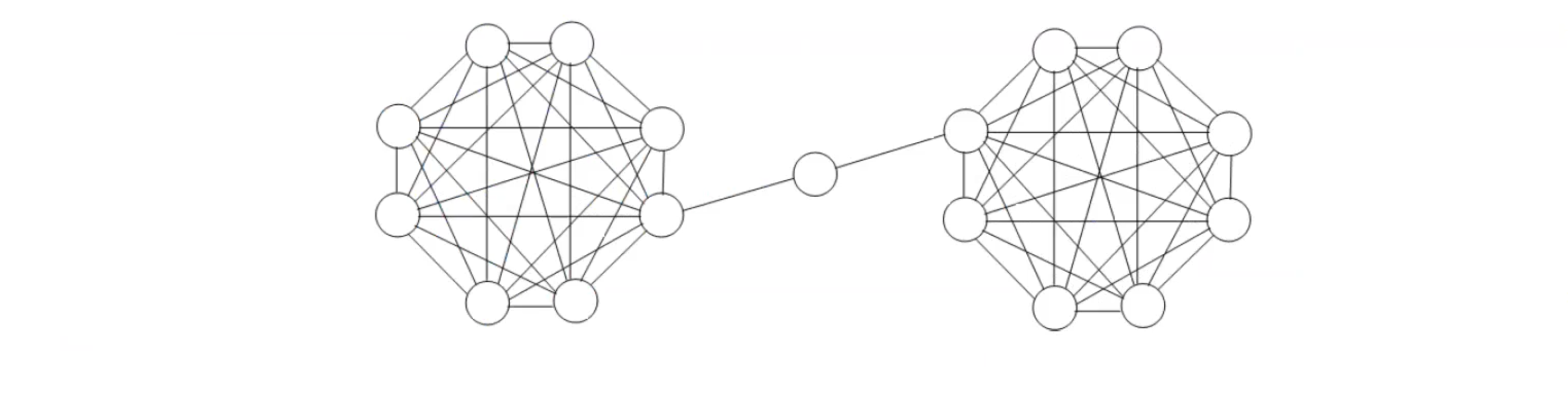
Betweenness centrality

Betweenness Centrality of node $i$ is calculated as the number of all shortest paths in the network that pass through $i$ .

$b_i={\sum }_{j,k}\frac{\text{n. of shortest paths connecting }j,k\mathrm{via}i}{\text{n. of shortest paths connecting }j,k}={\sum }_{j,k}\frac{n_{jk}(i)}{n_{jk}}$

Betweenness can be a valid and very useful property to consider in the computation of centrality in some models/networks.

Closeness centrality

A node is considered central if it is, on average, close to all the other nodes in a network. This means it has better access to information, more direct influence on other nodes, and so on. To calculate this average distance, we can use the formula:

$l_i=\frac{1}{N-1}{\sum }_j{d}_{ij}$

The closeness centrality is defined as

$c_i=\frac{1}{l_i}=\frac{N-1}{{\sum }_j{d}_{ij}}$

If the network is directed, we need to differentiate between in-closeness and out-closeness. If the network is weighted, there are several alternative definitions available for closeness centrality.

Eigenvector centrality

” I’m important if I’m friend of important people ”

It’s just called eigenvector because it’s computed using eigenvectors of the adjacency matrix. The centrality ${\gamma }_i$ is (proportional to) the sum of the centralities of the neighbours (i.e., a node is important if it relates to important nodes).

${\gamma }_i=\alpha {\sum }_j{a}_{ij}{\gamma }_j$

Letting $\gamma ={\left[\begin{array}{llll}{\gamma }_1& {\gamma }_2& \dots & {\gamma }_N\end{array}\right]}^T$ and $\lambda =1/\alpha$, we obtain the eigenvector equation:

$A\gamma =\lambda \gamma$

If the network is connected ( $=A$ is irreducible), the centralities ${\gamma }_i$ are given by the only solution with $\lambda >0,{\gamma }_i>0$ for all $i$ (Frobenius-Perron theorem).

• “Quantitative Sociologists” (who is the most influential individual?)
• applications in web searching (with some modifications: Google “PageRank” which is the most important webpage?)
• another modification is Katz (or alpha-) centrality: ${\gamma }_i=\alpha {\sum }_j{a}_{ij}{\gamma }_j+\beta$ just a variant to solve some degeneration problem of the eigenvector centrality in not completely connected networks.

Random walker centrality

${\pi }_{i,t}$ is the state probability, which means the probability of being in node $i$ at time $t$ :

${\Sigma }_i{\pi }_{i,t}=1\forall t$

With $t\to \infty$ we can define the centrality of node ${\pi }_i$ represents fraction of time spent on node $i$ by a random walker (only if the network is strongly connected). Basically this quantity/metric/centrality represents the frequency to find the random walker at node $i$.

“A node is important if is visited many times”

Random walker centrality is useless in undirected and unweighted networks ${\pi }_i$ since it is the rescaled node degree:

${\pi }_i=\frac{k_i}{{\sum }_j{k}_j}=\frac{k_i}{k_{tot}}$

In undirected but weighted networks:

${\pi }_i=\frac{s_i}{{\sum }_j{s}_j}=\frac{s_i}{s_{tot}}$

In directed networks, ${\pi }_i$ turns out to be mostly correlated to the in-strength $s_i^{in}$:

${\pi }_i=\frac{s_i^{in}}{{\sum }_j{s}_j}=\frac{s_i^{in}}{s_{tot}}$