06.Performance

Performance

Measuring the quality of a system is a classic engineering question.

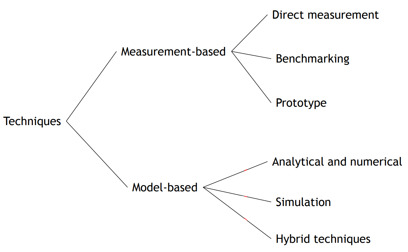
Possible models that we will se are:

• Queueing networks

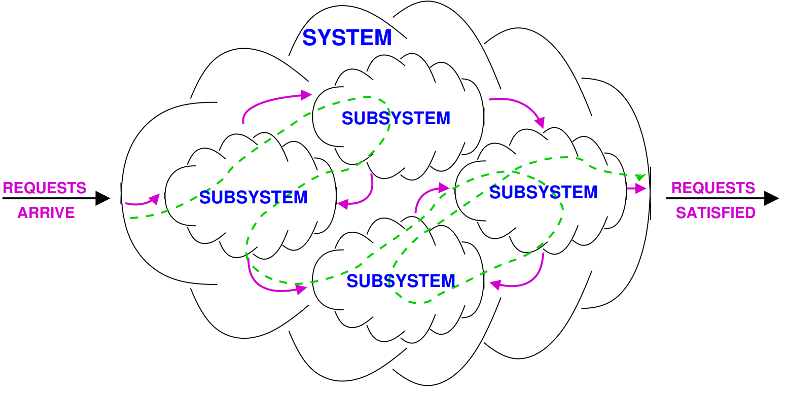
Queueing networks

Queueing theory is the theory behind what happens when you have a lot of jobs, scarce resources, and so long queue and delays. Examples of queues in computer systems:

• CPU uses a time-sharing scheduler
• Disk serves a queue of requests waiting to read or write blocks
• A router in a network serves a queue of packets waiting to be routed
• Databases have lock queues, where transactions wait to acquire the lock on a record

Different aspects characterize queuing models:

• Arrival: frequency of jobs is important: the average arrival rate $\lambda$ (req/s).
• Service: the service time is the time which a computer spends satisfying a job: the average duration $\frac{1}{\mu }$ and $\mu$ is the maximum service rate.
• Queue: jobs or customers which cannot receive service immediately must wait in a buffer.
• Population: we can both have members of the population indistinguishable or divided into classes, whose members differs in one or more characteristics, for example, arrival rate or service demand.
• Routing: the policy that describes how the next destination is selected after finishing service at a station must be defined. It can be:
  • probabilistic: random destination
  • round robin: the destination chosen by the job rotates among all the possible ones
  • shortes queue: jobs are moved to the one other subsystem with the mallest number of jobs waiting

{width=50%}

Operational laws

Operational laws represent the average behavior of any system, without assumptions about random variables. They are simple easy to apply equations.

If we observe a system we might measure these quantities:

• $T$ the length of time we observe the system
• $A$ the number of request arrivals we observe
• $\mathrm{C}$ the number of request completions we observe
• $B$ the total amount of time during which the system is busy $(B\le T)$
• $\mathrm{N}$ the average number of jobs in the system
• $R$ the average time a request remains in the system (also called residence time). It corresponds to the period of time from when a user submits a request until that user’s response is returned.
• ${\tilde{R}}_k$ of a sub-system $k$ is the response time and it’s the average time spent by a job in $k$ when enters the node.
• $Z$ is the think time which represents the time between processing being completed and the job becoming available as a request again, basically the time where in interactive systems the app is waiting the user.

From the quantities we can derive these equations:

• $\lambda =A/T$, the arrival rate
• $X=C/T$, the throughput or completion rate where $C$
• $U=B/T$, the utilization
• $S=B/C$, the mean service time per completed job. Note that is the average time that a job spends when IT IS SERVED.
• $U=XS$ which is useful in situations like “consider a serving rate of $x$ where each serving need $S$ time to be completed”.
• $N=XR$ which is called the little law.
• $R=\frac{N}{X}-Z$ in case of interactive systems.
• $V_k=\frac{C_k}{C}$ is the visit count of sub-system $k$ in the system with $C$ as completion rate. It’s possible that $C_k>C$ when there are “loops” in the model
• $C_k=V_{k}C$
• $X_k=V_{k}X$ is the force flow law and it captures the relationship between sub-system $k$ with the system.
• $D_k=V_k{S}_k$ is the service demand and it represents the total time that the $k$ sub-system is needed for a generic request. It’s a crucial characteristic of the sub-system/resource.
• ${\tilde{R}}_k$ is the time spent by a job in a service station, counting the queue time.
• $R_k=V_k{\tilde{R}}_k$ is the residence time and is the time spent by a job in a service station during all system time: so accounting the visits of the component.
• $U_k=D_{k}X$ is the utilization of a resource/sub-system.

If the system is job flow balanced $C=A$ which means that $\lambda =X$ . Also the above formulas can also be applied to a single sub system $k$.

Performance bounds

We only consider single class systems and determine asymptotic bounds on a system’s performance indices. Our focus will be on highlighting the bottleneck and quantify its impact.

The considered models and the bounding analysis make use of the following parameters:

• $K$, the number of service centers
• $D={\sum }_k{D}_k$
• $Dmax$, the largest service demand at any single center
• $Z$, the average think time, for interactive systems

And the following performance quantities are considered:

• $X$, the system throughput
• $R$, the system response time

We distinguish between open model and closed model.

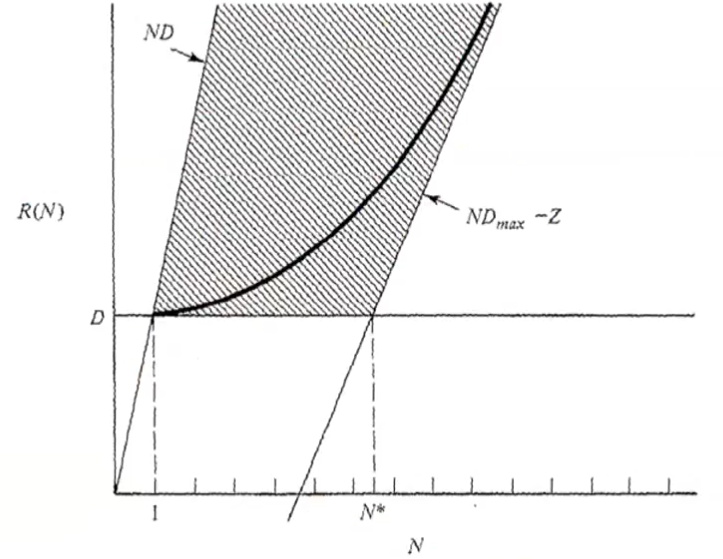
Open Models

In open models we have the following bounds:

$X(\lambda )\le \frac{1}{D_{\max }}$

which is essentially derived from these relations:

$$D_{\max }=\underset{k}{\max }{D}_k$$ $$U⩽1X\cdot D_k⩽1$$

And the for the response time: $D\le R(\lambda )$

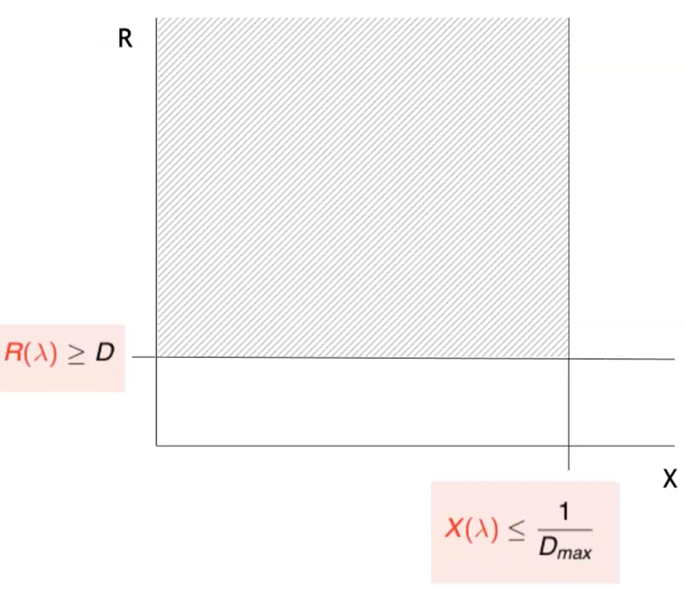
The upper bound for $R$ cannot be defined while minimum response time is the sum of all the demands of all components..

Closed models

$\frac{N}{ND+Z}\le X(N)\le \min \left(\frac{N}{D+Z},\frac{1}{D_{\max }}\right)$

$\max \left(D,N{D}_{\max }-Z\right)\le R(N)\le ND$

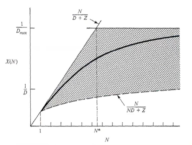
We can distinguish when the system is operating at “light load” from an heavy load.

• Light load: $\frac{N}{ND+Z}\le X\le \frac{N}{D+Z}$
• Heavy load: $\frac{N}{ND+Z}\le X\le D_{max}$