09.RL Techniques

RL Techniques

RL Techniques nomenclature

There are many distinctions in the RL techniques to approach the problem:

• Model-free vs. Model-based: RL doesn’t necessarily require a predefined model of the environment. During the RL process, the collected samples can be used in two main ways:

  • Model-based: to estimate the environment’s model.
  • Model-free: to estimate the value function without explicitly modeling the environment.

• On-policy vs. Off-policy: These terms refer to the relationship between the policy being learned and the policy used to collect samples:

  • On-policy: Learns the value function of the policy being enacted to collect samples. It involves playing the policy $\pi$ and learning its $Q$-function $Q^{\pi }$.
  • Off-policy: Learns the value function of a policy that is different from the one used to collect samples. It involves playing an exploratory policy while learning the optimal $Q$-function $Q^{\ast }$.

• Online vs. Offline: This distinction is based on how the RL system interacts with the environment:

  • Online: The system continuously interacts with the environment, updating its policy and collecting new samples in real-time.
  • Offline: The system relies on a fixed set of previously collected interaction data, with no further interaction with the environment.

• Tabular vs. Function Approximation: This refers to the method of storing the value function:

  • Tabular: The value function is stored in a table, with discrete states and actions.
  • Function Approximation: The value function is represented using a mathematical function, which can be a simple linear approximator or a complex neural network. This approach is particularly useful for dealing with continuous states and actions.

Prediction & Control

The are 2 concepts which form the foundation for the behavior of agents within an environment:

• Model-free prediction: estimate value function of an unknown MRP (MDP + fixed policy $\pi$). We will see:
  • Monte Carlo
  • Temporal Difference
• Model-free control: optimize value function of an unknown MDP to learn optimal policy. We will see:
  • Monte Carlo Control: Monte Carlo estimation of $Q^{\pi }(s,a)$ combined with $\epsilon$-greedy policy improvement
  • SARSA: Temporal Difference $\mathrm{TD}(0)$ estimation of $Q^{\pi }(s,a)$ combined with $\epsilon$-greedy policy improvement
  • Q-learning: empirical version of Value Iteration Off-policy: play an explorative policy and learn the optimal Q-function $Q\ast$

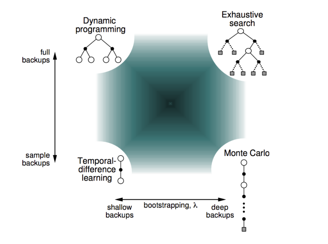
Monte Carlo

Monte Carlo is a simple approach for estimating the value function or Q(s,a) (if we are predicting or controlling) directly from experience by taking the mean of the return of observed episodes. However, it is not suitable for long episodes or infinite horizons.

Monte Carlo for prediction

Monte Carlo for prediction tasks blueprint:

• wait until the end of the episode
• only episodic problems
• high variance, zero bias
• Good convergence properties
• not very sensitive to initial values
• adjust prediction toward the outcome
• general approach, less efficient

It comes in two flavors (First-Visit vs. Every-Visit) where the main difference lies in how they handle repeated visits to states within episodes:

In first-visit Monte Carlo, only the first visit to a state in an episode is used for the value estimate, avoiding bias towards states visited more frequently. Every-visit Monte Carlo, however, includes all visits to a state within an episode, introducing a bias towards more frequently visited states.

Monte Carlo for control

Monte Carlo methods extend to control tasks, where the goal is to optimize the policy:

• Generalized Policy Iteration: The control approach follows a similar two-step process of policy evaluation and improvement, but adapted for the RL context where the model is unknown.
• Policy Evaluation: Monte Carlo is used to evaluate the Q(s, a) function for the current policy, providing a basis for policy improvement.
• Policy Improvement: A greedy improvement is made over Q(s, a) to enhance the policy. However, a purely greedy policy would lack exploration.
• $ϵ$-Greedy Exploration: The idea is “never give 0 probability to any action”. To ensure exploration, the deterministic policy is modified to select a random action with probability $ϵ$, while choosing the greedy action with probability $1-ϵ$. The parameter $ϵ$ regulates the amount of exploration. There is an equivalent policy improvement theorem also for $ϵ$-greedy policies, so we are sure that the resulting policy is always an improvement.

Temporal Difference

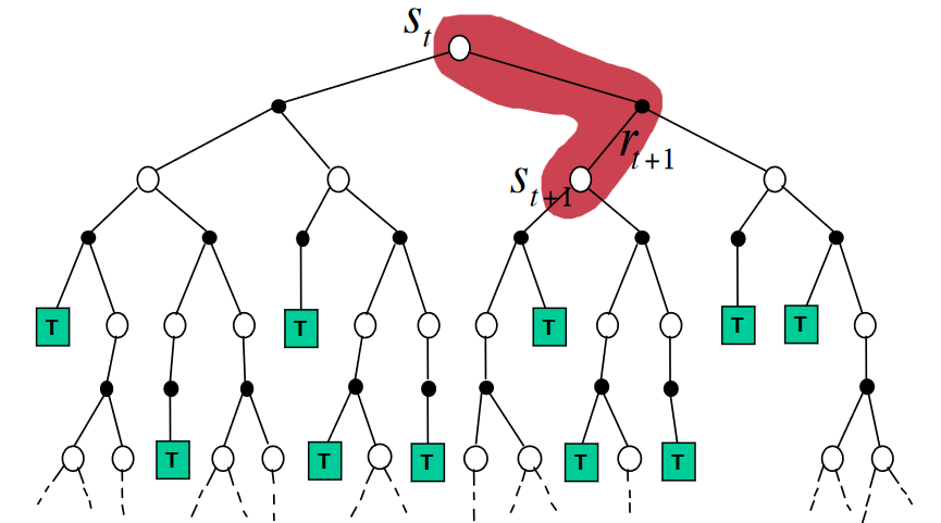
Temporal Difference (TD) learning method is a crucial technique in RL. At the heart of this method lies the update equation:

$V\left(s_t\right)\leftarrow V\left(s_t\right)+\alpha \left(r_{t+1}+\gamma V\left(s_{t+1}\right)-V\left(s_t\right)\right)$

• $r_{t+1}$ represents the immediate reward received after transitioning from state $s_t$ to state $s_{t+1}$.
• Finally, $(r_{t+1}+\gamma V(s_{t+1})-V(s_t))$ calculates what’s known as TD error (Temporal Difference error). It measures the difference between our current estimate of the value of being in state $s_t$, i.e., $V(s_t)$, and our updated estimate using new information about rewards obtained from transitioning from state $s_t$ to state $s_{t+1}$.

TD for prediction

RL version of the Bellman expectation equation. TD can bootstrap that is it can learn from incomplete episodes. Temporal difference uses its previous estimation to update its estimation (biased but consistent).  

Blueprint of TD:

• Usually more efficient than MC
• learn online at every step
• can work in continuous problems
• low variance, some bias
• worse for function approximation
• more sensitive to initial values
• adjust prediction toward next state
• exploits the Markov properties of the problem

TD($\lambda$)

TD($\lambda$) represents an advanced Temporal Difference (TD) learning which harmonizes the concepts of TD that span from immediate TD updates to the episode-encompassing Monte Carlo ones.

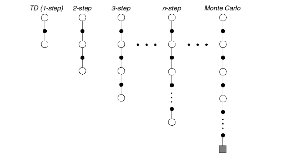
Basically it’s an intermediate approach between TD and MC.

$$V\left(s_t\right)\leftarrow V\left(s_t\right)+\alpha \left(v_t^{\lambda }-V\left(s_t\right)\right)$$

The parameter $\lambda$ regulates how much we lean towards an approach or the other and the bias-variance trade-off. In MC we look at all the steps while TD ($TD(0$)) looks only at one step. $TD(\lambda )$ looks at some steps into the future before using the approximation.  

• n = 1 is the temporal difference approach ($TD(0)$)
• n infinite is the Monte Carlo approach

TD for control

D Control algorithms iteratively adjust the Q-values, which represent the expected returns of taking a particular action in a given state and following a specific policy thereafter. By optimizing these Q-values, the algorithms effectively refine the agent’s policy towards the optimal strategy for maximizing rewards over time. The most notable TD Control algorithms include:

• SARSA (State-Action-Reward-State-Action)
• Q-Learning

SARSA algorithm

This is an on-policy TD control algorithm where the agent learns the Q-value based on the action taken under the current policy. SARSA updates its Q-values using the equation:

$Q\left(s_t,a_t\right)\leftarrow Q\left(s_t,a_t\right)+\alpha \left(r_{t+1}+\gamma Q\left(s_{t+1},{\mathbf{a}}_{\mathbf{t}+1}\right)-Q\left(s_t,a_t\right)\right){\mathbf{a}}_{\mathbf{t}+1}\sim \pi \left(\cdot \mid s_{t+1}\right)$

SARSA $\lambda$ extends the SARSA algorithm by incorporating the ideas from $TD(\lambda )$, effectively creating a bridge between SARSA($0$) and Monte Carlo methods.

SARSA($\lambda$) strikes a balance in information propagation between:

• SARSA: Updates only the latest state-action pair, limiting the scope to immediate transitions.
• Monte Carlo (MC): Updates all visited pairs in an episode, considering the full sequence of actions.
• SARSA($\lambda$): Blends both approaches, updating recent and past pairs with diminishing impact via eligibility traces, ensuring a balance between immediate and comprehensive updates.

Q-learning

Q-learning seeks to learn the optimal policy even when the agent is not following it. The Q-value update rule for Q-learning is:

$(Q(s,a)\leftarrow Q(s,a)+\alpha [r+\gamma {\max }_{a^{\prime }}Q(s^{\prime },a^{\prime })-Q(s,a)])$

where $({\max }_{a^{\prime }}Q(s^{\prime },a^{\prime }))$ represents the maximum $Q$-value for the next state $s^{\prime }$ across all possible actions $a^{\prime }$.

Q-learning will learn the optimal policy even if it always plays the random policy. The only requirement is that we need to have a policy that have non zero probability to each action, but there is no constraint on the policy.

Why is this important?

• learn by observing someone else behavior
• reuse experience generated from old policies
• learn about multiple policies while following one policy

So the important difference between Q-learning and SARSA is that SARSA is an on-policy approach and can only learn the best $ϵ$-greedy policy considering also the exploration.