03.Frequency Domain

Frequency Domain

Transfer functions

The transfer function $W(z)$, being a ratio of two polynomials, acts as a digital filter. It is instrumental in transforming $WN$ into an ARMA process and is applied in analyzing stationary processes through digital filter theory.

Shift Operators in Time Domain Analysis

• Backward shift operator $z^{-1}$ shifts a signal back in time
• Forward shift operator $z$ shifts a signal forward in time.

Properties of $z$ and $z^{-1}$ include linearity, recursive application, and linear composition. Using these properties, we can rewrite an AR model equation in terms of $z$ and $z-1$, revealing the relationship between the operators and the AR model. The resulting equation shows that the output $y_t$ is the ratio of two polynomials of $z$:

$y(t)=\frac{c_0+c_1{z}^{-1}+\cdots c_n{z}^n}{1-a_1{z}^{-1}+\cdots a_m{z}^{-m}}e(t)=\frac{C_{(z)}}{A(z)}e(t)=W(z)e^{it}(t)$

Asymptotically stability

Stability analysis involves examining the poles of the transfer function:

$y(t)=\frac{C(z)}{A(z)}e(t)$

• Zeros are values of $z$ where the transfer function equals zero
• Poles are the inverse of the transfer function’s roots (roots of $A(z)$ in case of no cancellations).

The locations of poles and zeros, particularly within the unit circle in the complex plane, are indicative of system stability.

• To compute zeros, set the numerator of the transfer function equal to zero.
• For poles, set the denominator equal to zero.

A system is considered asymptotically stable if all poles lie strictly inside the unit circle, and it is deemed a minimum phase system if both poles and zeros reside within the unit circle.

The asymptotic stability is often necessary to demonstrate if a process $y(t)=W(z)e(t)$ is stochastic process:

• the process transfer function is asymptotically stable (its poles are all located within the unitary circle)
• the input (e.g. $e(t)$) is a stationary stochastic process

Canonical representation of $SSP$

Stationary stochastic processes (so including ARMA, MA and AR) can be equivalently represented in 4 distinct ways, each offering unique insights and applications:

Probabilistic representation:

$y(t)=m_y,{\gamma }_y(\tau )$ the mean provides information about the central tendency of the process, while the covariance function captures how data points at different time lags are related: particularly useful for understanding the process’s statistical properties and for generating simulations.

Difference equations (time domain):

$y(t)=a_{1}y(t-1)+\cdots a_{m}y(t-m)+c_{o}e(t)+\cdots c_{n}e(t-n)$

essential in modeling and forecasting

Transfer function (operatorial):

$y(t)=\frac{C(z)}{A(z)}e(t)$ Transfer functions are commonly used in control theory and engineering applications, where the focus is on manipulating and controlling the process.

Frequency

$y(t)=m_y,{\Gamma }_y(\omega )$It is especially valuable in applications involving signal processing, where the focus is on understanding the frequency content of the data.

They are all equivalent but not unique. The uniqueness aspect it will be problematic, and so before introducing prediction theory, we need to better understand the non-uniqueness property and find ways to make the representation unique.

Taken the process in operatorial representation:

$y(t)=\frac{C(z)}{A(z)}e(t)$

We can adopt this “convention” to be sure about the uniqueness of representation:

1. monic: the term with the highest power has coefficient equal to $1$
2. coprime: no common factors to that can be simplified
3. have same degree
4. have roots inside the unit circle

The spectral factorization theorem

In the analysis of discrete-time signals through the use of the transfer function $W(z)$, if $y(t)=W(z)v(t)$ and:

• $v(t)$ is stationary
• $W(z)$ is stable

$y(t)$ is well defined and stationary.

Final value theorem

The final value theorem or theorem of the gain is:

$E[y(t)]=W(1)\cdot E[u(t)]$

NB: The final value theorem can be applied to $W(z)$ that are not in canonical form.

Final value theorem is useful when we want to define de-biased process:

1. Find mean with gain theorem: $E[y(t)]=W(1)\cdot \mu =\bar{y}$

2. Define de-biased processes:

   $$\begin{array}{rl}\tilde{y}(t)& =y(t)-\bar{y}\\ \tilde{e}(t)& =e(t)-\mu \end{array}$$

3. Do whatever you want, like computing the covariance ${\gamma }_{\tilde{y}}(\tau )={\gamma }_{\gamma }(\tau )\forall \tau$

All Pass Filter

In the context of transfer functions $W(z)$ and digital filters, an all pass filter is a particular process which transform a white noise in a white noise with a different variance.

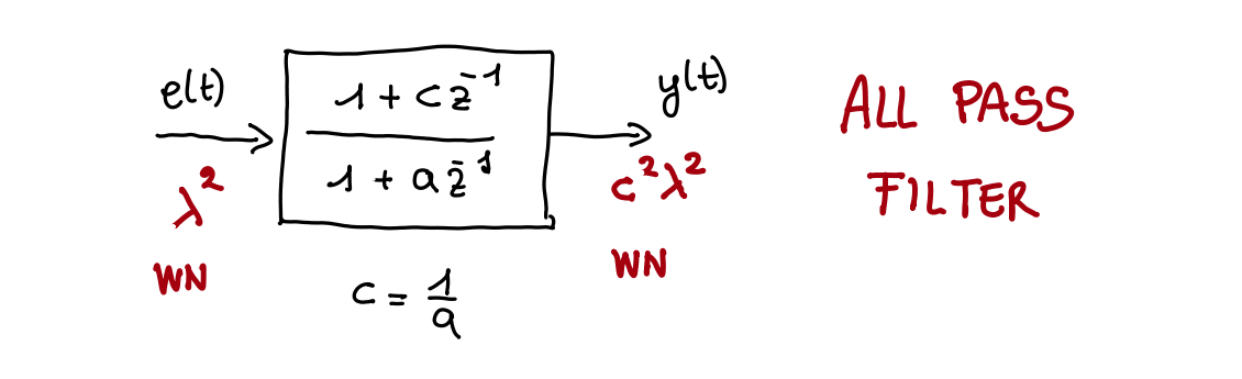
An APF is useful for converting a system to canonical form: we can do this by aggregating coefficients and multiplying by a fraction of identical polynomials (so that we essentially multiply by one) and then we redefine a new white noise process.

Apart the variance everything remains the same; for example if input $u(t)$ and output $y(t)$:

• If $u(t)$ is constant, $y(t)$ is constant.
• If $u(t)$ is sinusoidal, $y(t)$ is sinusoidal.

Spectral representation

Spectral density of a stationary stochastic process

${\Gamma }_y(w)={\sum }_{\tau =-\infty }^{\infty }{\gamma }_y(\tau )\cdot e^{-jw\tau }$

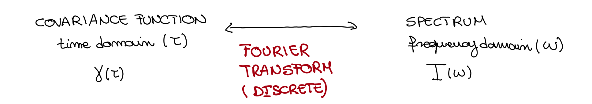
For a stationary process $y(t)$, ${\Gamma }_y(\omega )$:

• positive
• real
• even $\Gamma (-\omega )=\Gamma (\omega )$
• periodic with period $T=2\pi$.

Its graph can be represented in the upper half plane of a 2D plot, as the imaginary part is always zero.

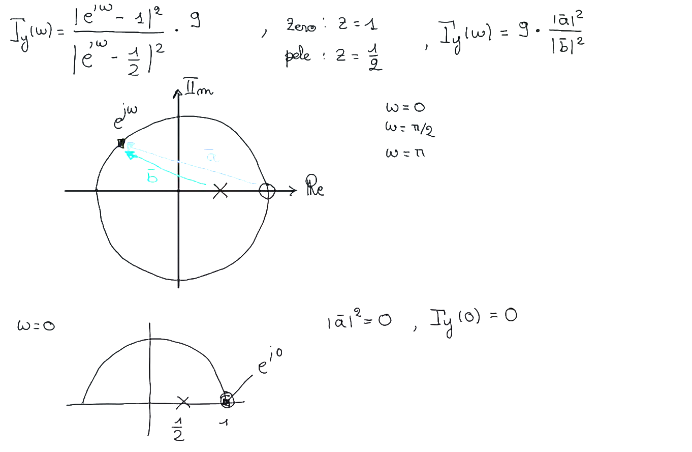
The “general rule” regarding the effect of the poles and zeros of the transfer function is that if the generic point $e^{j\omega }$ is:

• Near zeroes, the ${\Gamma }_y(\omega )$ exhibits attenuation. For a zero on the unit circle there is the so called blocking property of the transfer function, which refers to the phenomenon where a zero on the unit circle in the z-domain causes the system to completely attenuate that specific frequency component of the input signal. As the frequency moves away from this zero, the attenuation decreases.
• Near poles, the ${\Gamma }_y(\omega )$ is high. The frequency response is amplified. If a pole is near the unit circle, it signifies a strong frequency response at the angle $\omega$ corresponding to the pole’s position.

Spectrum Properties

For stationary processes, the following properties hold for the power spectral density $\Gamma (\omega )$:

1. Scalar Multiple If $y(t)=ax(t)$, then: $${\Gamma }_y(\omega )=a^2{\Gamma }_x(\omega )$$
2. Sum of Uncorrelated Processes: If $z(t)=x(t)+y(t)$ and $x(t)$ and $y(t)$ are uncorrelated, then: $${\Gamma }_z(\omega )={\Gamma }_x(\omega )+{\Gamma }_y(\omega )$$
3. Inverse transform returns the covariance function based on the spectral density, noted as the inverse discrete Fourier transform.

${\gamma }_y(z)=F^{-1}({\Gamma }_y(\omega ))=\frac{1}{2\pi }{\int }_{-\pi }^{\pi }{\Gamma }_y(\omega )d\omega$ 4. The spectrum of a $WN$ is constant and equal to its variance:

${\Gamma }_e(\omega )==Var[e(t)]={\lambda }^2$

Example

If $v(t)=ax(t)-by(t)$ and $x(t)$ and $y(t)$ are uncorrelated, then: ${\Gamma }_v(\omega )=a^2{\Gamma }_x(\omega )+b^2{\Gamma }_y(\omega )$

Fundamental theorem of spectral analysis

Very useful theorem to compute the spectrum:

${\Gamma }_y(\omega )=W(z=e^{j\omega })W(z=e^{-j\omega }){\Gamma }_u(\omega )$

It’s possible to apply the fundamental theorem of spectrum analysis also if $W(z)$ is not in the canonical form :)

Recall of useful formulas for spectrum qualitative study are:

• $e^{j\omega }=\cos \omega +j\sin \omega$
• $e^{-j\omega }=\cos \omega -j\sin \omega$
• $e^{-j\omega }+e^{+j\omega }=2\cos (\omega )$

Remember that is always possible to write the spectral density function as a real-valued function composed by cosine terms easier to interpret.