04.Model Prediction

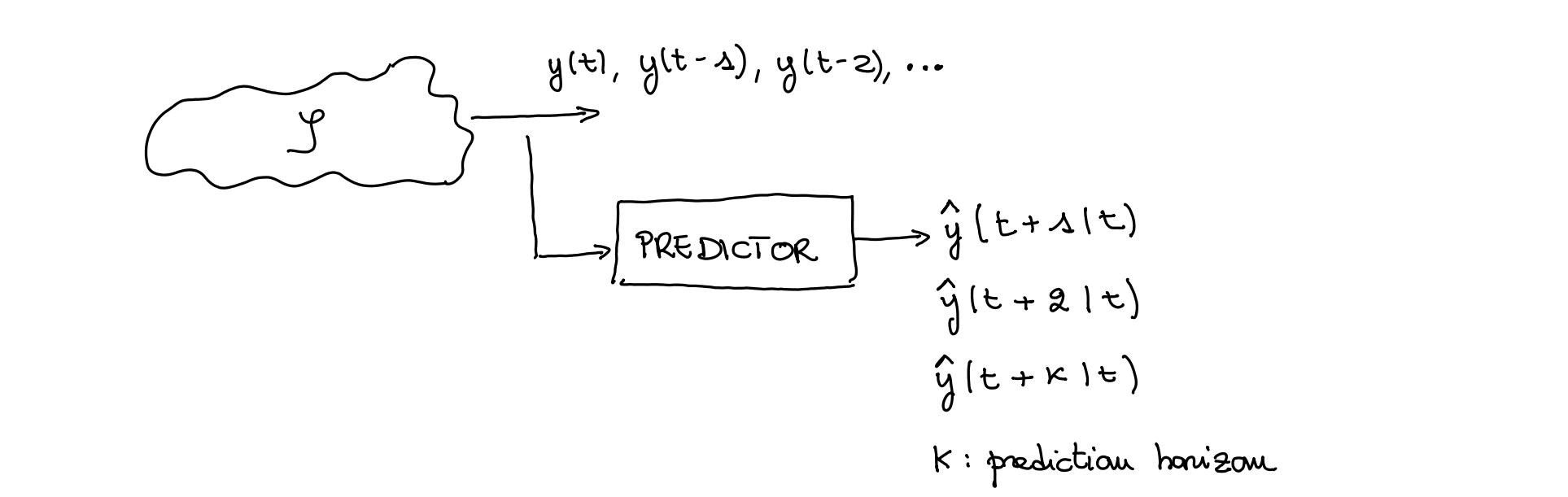
Model prediction

We want to find the predictor $\hat{y}(t)$ of process $y(t)$ from the past values of $y$.

Steps:

0. analysis of the system
1. evaluation of the canonical representation of the system
2. computation of the predictor
3. evaluate the prediction error

Practically the optimal predictor from data is:

$\hat{y}(t+n|t)=\frac{F(z)}{C(z)}y(t)$

This because:

$W(z)=\frac{C(z)}{A(z)}=\text{long division}=E(z)+\frac{z^{-u}F(z)}{A(z)}$ where $E(z)$ is the result of the long division, while $F(z)$ is the rest.

So:

$y(t+k)=\frac{C(z)}{A(z)}e(t+k)=\left[E(z)+z^{-k}\frac{F(z)}{A(z)}\right]e(t+k)$

In practice what happens is that the $E(z)e(t+k)$ part will be always be discarded and treated as the prediction error, while this $z^{-k}\frac{F(z)}{A(z)}e(t+k)$ can be use. So remember:

$ϵ(t)=E(z)e(t)$ It’s also interesting that since for the optimal 1-step predictor $E(z)=1$ , $ϵ(t|t-1)=e(t)$ always.

Actually to be used the predictor with respect to the data we will use this $e(t)=\frac{A(z)}{Cz}y(t)$ to re-write the equation into:

$\hat{y}(t+n|t)=\frac{F(z)}{A(z)}e(t)=\frac{F(z)}{A(z)}\cdot \frac{A(z)}{C(z)}\cdot y(t)=\frac{F(z)}{C(z)}y(t)$

Considerations:

• $\hat{y}(t+k,s)$ is a stochastic process, stationary (because the denominator $C(z)$ still has roots inside the unit circle).
• The quality of the prediction get worse with increasing $k$.
  • For $k=1$ the variance of the error coincides with the variance of the white noise
  • For $k\to \infty$ the variance of the error coincides with the variance of the process and the predictor becomes the expected value of the process

$var[e(t)]\le var[ϵ(t|t-k)]<var[y(t)]$

Canonical form in order to derive the optimal predictor

Apart removing the ambiguity and computational efficiency, the canonical form is important because:

• Stability: The canonical form ensures that the process is stable, which is a prerequisite for meaningful prediction.
• Whitening Filter: The canonical form implicitly defines a whitening filter:

$e(t)=\frac{A(z)}{C(z)}y(t)$ inverting this transformation is crucial for prediction to find the optimal predictor.

Remember: if it’s not in canonical form → non stable transfer function → so a non stationary predictor → the predictor is divergent.

So what we have to do is we have to do an intermediate step before, which is to take this into equivalent process description (the easiest way is to multiply by APF).

1-step predictor

If you use the formula previously presented for a 1 step ARMA predictor with null mean you will always obtain $E(z)=1$. This aspect permits to make some simplification in the final formula and just use these “shortcuts”:

$\hat{y}(t|t-1)=\frac{C(z)-A(z)}{A(z)}e(t)$ from data:

$\hat{y}(t|t-1)=\frac{C(z)-A(z)}{C(z)}y(t)$ And since:

$ϵ(t|t-1)=y(t)-\hat{y}(t|t-s)=y(t)-\frac{C_m-A_m}{C_m}y(t)=\left(\frac{C_m-C_m+A_m}{C_m}\right)y(t)$ the prediction error will always be: $ϵ(t|t-1)=\frac{A_m(z)}{C_m(z)}\cdot y(t)$

AR

The usual $AR(1)$ process: $v(t)=av(t-1)+\eta (t)$

The transfer function is: $W(z)=\frac{1}{1-a{z}^{-1}}$ So the optimal 1-step ahead predictor is: $\hat{v}(t|t-1)=\frac{a}{z}v(t)=av(t-1)$ With the optimal 2-steps ahead predictor we can see that:

$\hat{v}(t|t-2)=\frac{a^2}{z^2}v(t)=a^{2}v(t-2)$

By generalization we can say that for an $AR(1)$ process the optimal predictor is always: $\hat{v}(t+r|t)=a^{r}v(t)$

Another notorious predictor is that for $AR(n)$ the 1-step predictor will be always:

$\hat{v}(t|t-1)=a_{1}v(t-1)+a_{2}v(t-2)\dots a_{n}v(t-n)$

ARMA with not null mean

Remember that for processes with non-null term we have some troubles? Also when computing predictors with not null mean we have to make some sbatti:

$\begin{array}{rl}y(t+k)& =\hat{y}(t+k)+my\\ \hat{y}(t+k|t)& =\hat{y}(t+k|t)+my\end{array}$

To make the predictor we have to just consider the unbiased process, so first of all compute the mean with gain theorem:

$E[y(t)]=W(1)\cdot \mu =my$

Then define de-biased processes:

\tilde{y}(t) &= y(t) - my \\ \tilde{e}(t) &= e(t) - \mu \end{aligned}$$ Redefine the process using unbiased elements: $$ \tilde{y}(t+k|t) = \frac{C(z)}{A(z)} \cdot \tilde{e}(t)$$ And apply the generic formulas for the predictor. At the end we can make the prediction adjustment for non-zero-mean: $$ \hat{y}(t+k|t) = \tilde{y}(t+k|t) + my $$ $$\begin{aligned}\hat{y}(t+k|t)&=\frac{F(z)}{C(z)}\tilde{y}(t)+my=\frac{F(z)}{C(z)}(y(t)-my)+my\\&=\frac{F(z)}{C(z)}y(t)-\frac{F(z)}{C(1)}my+my\end{aligned}$$ and the final formula is: $$ \hat{y}(t+k|t) = \frac{F(z)}{C(z)} \cdot y(t) + \left(1 - \frac{F(1)}{C(1)}\right) \cdot my $$ ## ARX and ARMAX We want to predict the generic ARMAX process: $$y(t)=\frac{C(z)}{A(z)}e(t)+\frac{B(z)}{A(z)}u(t-d)$$ where $d$ is the pure delay. The ARMAX predictor from data: $$\widehat{y}(t|t-k)=\frac{F_{k(z)}}{C(z)}y(t-k)+\frac{B(z)E(z)}{C(z)}u(t-d)$$ The ARMAX 1-step predictor ($E(z)=1$) from data: $$\widehat{y}(t|t-1)=\frac{C(z)-A(z)}{C(z)}y(t-1)+\frac{B(z)}{C(z)}u(t-d)$$ ### Demonstration Assuming already canonical $\frac{C(z)}{A(z)}$ and $u(t)$ known process (so completely **deterministic**) we only need predictor for stochastic part. Said this we compute the predictor in a similar way as before: $$y(t)=\frac{C(z)}{A(z)}e(t)+\frac{B(z)}{A(z)}u(t-d)$$ Now, let's consider the long division between $C(z)$ and $A(z)$: $$\dfrac{C(z)}{A(z)}=E(z)+\frac{F(z)}{A(z)}$$ Which can be written as: $$A(z)=\frac{C(z)-F(z)}{E(z)}$$ Let's put it in the ARMAX equation: $$\left(\frac{C(z)-F(z)}{E(z)}\right)y(t)=C(z)e(t)+B(z)u(t-d)$$ Let's rewrite it as: $$C(z)y(t)=F(z)y(t)+C(z)E(z)e(t)+B(z)E(z)u(t-d)$$ Let's divide by $C(z)$: $$y(t|t-k)=\frac{F(z)}{C(z)}y(t-k)+\frac{B(z)E(z)}{C(z)}u(t-d)+E(z)e(t)$$ Last term as usual is unpredictable at time $t-k$ : $$\widehat{y}(t|t-k)=\frac{F_{k(z)}}{C(z)}y(t-k)+\frac{B(z)E(z)}{C(z)}u(t-d)$$