06.Model validation

Model validation

Given an optimal model $M({\hat{\theta }}_n)$ the goal is to validate its optimality also considering its model order $n.$ Using measured samples, one can estimate the prediction error variance through $J_k(a)$, which evaluates the performance of the predictive model:

$J_k(a)=\frac{1}{k}{\sum }_{t=0}^{t=k}{\left(y(t+1)-\hat{y}(t+1|t)\right)}^2$

At the end we can say that even with measured samples (so finite data) asymptotically we will converge to the minimum of the asymptotic cost since: $J_N(\vartheta )\underset{N\to \infty }{\to }\bar{J}(\vartheta )=\mathbf{E}[{\epsilon }_{\vartheta }(t{)}^2]$ which implies that:

$\min \{J_N(\vartheta )\}\underset{N\to \infty }{\to }\min \{\bar{J}(\vartheta )\}$

PEM converges to real $S$

Now let’s prove that when the model set incorporates the actual dynamics of the system, the identified model using the prediction error method converges to the precise representation of the real system.

More formally, let’s prove that if $S\in M(\theta )$ PEM guarantees that $M({\hat{\theta }}_N)\to S$ or alternatively let’s prove that ${\theta }^oϵ\Delta$.

$\begin{array}{rl}& \epsilon (t|t-1,\theta )=y(t)-\hat{y}(t|t-1,\theta )\\ & =y(t)-\hat{y}(t|t-1,{\theta }^0)+\hat{y}(t|t-1,{\theta }^0)-\hat{y}(t|t-1,\theta )\end{array}$ $\begin{array}{r}\mathbb{E}[\epsilon (t|t-1,\theta {)}^2]=\mathbb{E}[(e(t)+\hat{y}(t|t-1,{\theta }^0)-\hat{y}(t|t-1,\theta ){)}^2]=\\ E[e(t{)}^2]+E[(\hat{y}(t|t-1,{\theta }^0)-\hat{y}(t|t-1,\theta ){)}^2]+0\\ ={\lambda }^2+0\end{array}$

Last passage is possible since $\theta ={\theta }^0$ in the case of the global optimum (as said above, PEM is guarantee to converge to the minimum of the asymptotic cost so $\theta ={\theta }^0$).

This theorem is very, very significant: if the system that you want to model and learn from data is inside the model set, you will converge asymptotically (so with a large data set) to exactly that system.

${\hat{\theta }}_N\underset{N\to \infty }{\to }{\theta }^o$

It means that the prediction error algorithm that we are using in this course is actually good, meaning that they will lead you to the right model (at least in this very ideal case where the system is in the model set).

Actually it’s very rare that $S\in M(\theta )$.

Let’s summary the possible cases:

• $S\in M(\theta )$ and $\Delta$ is a singleton : for $n\to \infty$ $M({\hat{\theta }}_n)$ will converge to $S$. The identification problem is properly defined, ensuring a singular, accurate solution that aligns with the system’s dynamics.
• $S\in M(\theta )$ and $\Delta$ is not a singleton : for $n\to \infty$ $M({\hat{\theta }}_n)$ will not necessary converge to $S$, but it’s guarantee ${\hat{\vartheta }}_N$ tends to one of the values in $\Delta$ (multiple optimal minima subset). Multiple models equally represent the system.
• $S\notin M(\theta )$ and $\Delta$ is a singleton: for $n\to \infty$ $M({\hat{\theta }}_n)$ will converge to $M({\theta }_n^{\ast })$. In this case the model with ${\hat{\vartheta }}_N$ is the best proxy of the true system in the selected family. There is an insufficiency of the model set to capture the system’s complexity.
• $S\notin M(\theta )$ and $\Delta$ is not a singleton: for $n\to \infty$ $M({\hat{\theta }}_n)$ no guarantees. In this case the model with ${\hat{\vartheta }}_N$ tends to one of the best proxies of the true system in the selected family. The model is too complex for the model or the data are not representative enough, basically we don’t know how to choose in a set of equivalent models.

Model order selection

How can we select the best value of $n$ namely the best model complexity? Remember that $J_n^n(\theta )$ in function of $n$ is always non increasing but it’s not the optimal predictor!

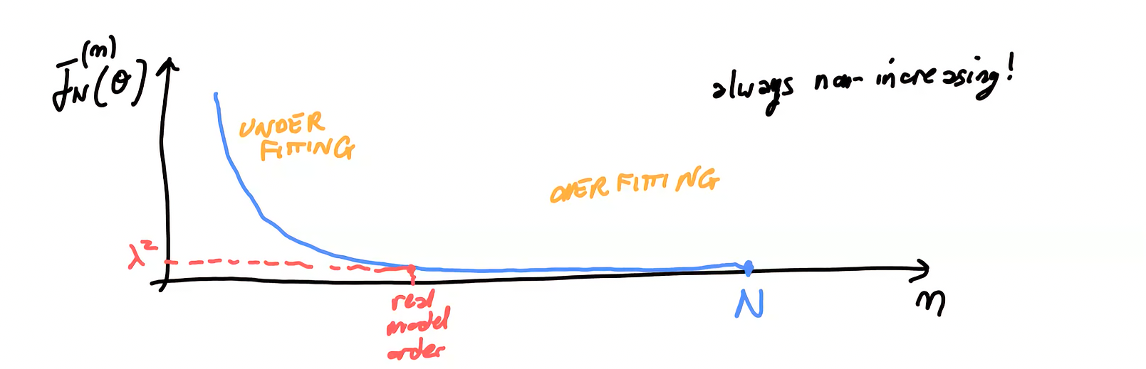
So in general an $ARX(n,n)$ is a better fit to the data than an $ARX(n-1,n-1)$ model, but we can’t simply continue to use more parameters, we would overfit it.

Whiteness test on residuals

If we simply compute the performance index for multiple increasing values of $n$ we will see that is monotonically decreasing with $n$: we can use the whiteness test on residuals to understand when “it’s enough” and that further decreasing will not reflect in better performance for new unseen data (overfit).

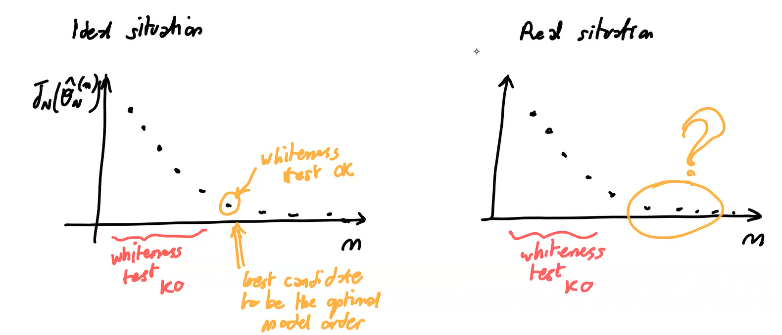
Actually this method is not robust and it’s not used.

Cross-validation

In cross-validation, the dataset is partitioned into an identification set (or training), which is used to construct the model, and a validation set, which is utilized to assess the model’s performance. The validation portion of the data is “reserved” and not used in the model-building phase, potentially leading to data “wastage”.

Identification with model order penalties

For better model selection that help prevent over-fitting we can directly control model complexity.

FPE (Final Prediction Error)

Identification with model order penalties:

$FPE=\frac{N+n}{N-n}{J}_N({\hat{\theta }}_N{)}^{(n)}$

We are giving a penalty to the models with high complexity. The FPE functions is not monotonically decreasing, and the complexity corresponding to its minimum value can be chosen as complexity of the model.

AIC (Akaike Information Criteria)

$AIC=\frac{2N}{n}+\ln \left(J_N({\hat{\theta }}_N{)}^{(n)}\right)$ For high values of $N$, this is equivalent to $FPE$.

MDL (Minimum Description Length)

Asymptotically is similar to AIC but with higher penalization since $ln(N)>2$ . $MDL=\ln (N)\frac{n}{N}+\ln \left(J_N({\hat{\theta }}_N{)}^{(n)}\right)$ In general case $S\notin M(\theta )$ we usually prefer to (slightly) overfit, so generally AIC is preferred.